Why Size is a Continuous Variable

Sample Size – Measuring a Continuous Variable

Introduction

When planning a test on a continuous variable, the most common question was "How many should I test"? Later, when the test results were available, the questions were "What is the confidence?" or "How precise was the result?" This article focuses on planning the measurements of a continuous variable and analyzing the test results.

Definition

A continuous variable is a variable that has an infinite number of possible values. This contrasts with a discrete variable which can take on a finite number of values. Examples of continuous variables would be dimensions, weight, electrical parameters, plus many others.

The Data

Let's assume we want to determine the value for a characteristic. There are parts available to measure so we take one measurement per part. The measurements are close, but don't agree.

If the data is plotted in a frequency histogram, generally there is a pattern that shows a center and variation about the center. Usually the data exhibits the bell curve indicative of a normal distribution. Since the center appears is a common value, but the center value changes with each sample of parts. We need a simple statement of the value of the center, some measure of the measurement accuracy, and some confidence in the results.

The Central Limit Theorem

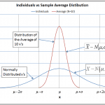
In another article, I discussed "The Central Limit Theorem", which states that the data average is approximately normally distributed even if the data distribution is non-normal. A comparison of normally distributed x's and the distribution of averages of 10 x's is shown graphically, figure 1.

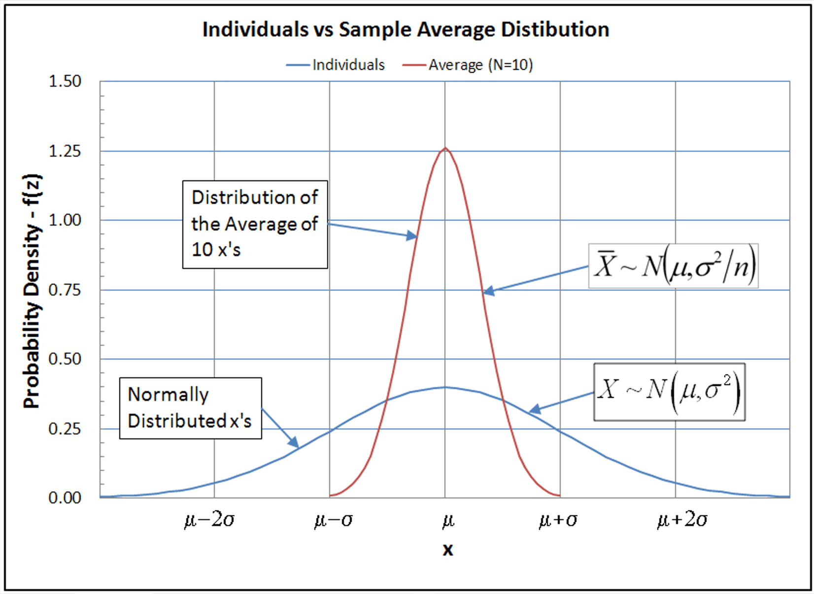
Figure 1

Note, that the distribution of the average is much narrower than the distribution of the individuals. When X is normally distributed about a mean μ with standard deviation σ, a short hand notation used by statisticians is $-X\sim N(\mu,\sigma^2)-$. Here N indicates the normal distribution, not sample size. Then, the distribution of the averages of size n is $-\bar{X}\sim N(\mu,\sigma^2/n)-$.

The sample statistics and S provide estimates of the population parameters μ and σ, where

$$\bar{X}=\frac{1}{n}\sum_{i=1}^{i=n}X_i$$

(1)

and

$$S^2=\frac{1}{n-1}\sum{(X_i-\bar{X})^2}$$

(2)

The Math

Both $-\bar{X}-$and S are subject to sampling variation. We don't know the distribution of $-\bar{X}-$about μ because we don't know μ and σ.In my article "Estimating Normal Distribution Parameters and Tolerance Limits", it was shown that the distribution of μ values follow a t-distribution. The appropriate probability statement is

$$Pr(\bar{X}+t_{\alpha/2,n-1}<\mu<\bar{X}+t_{1-\alpha/2,n-1})=1-\alpha$$

(3)

The tolerance interval is on μ is $-(\bar{X}+t_{\alpha/2,n-1},\bar{X}+t_{1-\alpha/2,n-1})-$. This interval looks odd, but it is a consequence of the fact that when α<0.5, the values of t are negative.

A tolerance is desired to contain $-\mu-$ within $-\pm\Delta-$ of $-\bar{X}-$, expressed as

$$\bar{X}\pm\Delta$$

(4)

When C is specified, then the appropriate significance level is $-\alpha=1-C-$. The tolerance Δ is determined using equation 3.

$$\Delta=t_{1-\alpha/2,n-1}S/\sqrt{n}=-t_{\alpha/2,n-1}S/\sqrt{n}$$

(5)

From equation 5, Δ is proportional to S, decreases with increasing sample size, and increases if higher confidence is desired. Equation 5 can be rearranged to form the equation 6.

$$n=(t_{\alpha/2,n-1}S/\Delta)^2$$

(6)

Equation 6 is a difficult to solve since n occurs in both sides of the equation. The calculation may require an iterative process to determine the best possible value. When test sample sizes are large, the value of the $-t_{\alpha/2,n-1}-$statistic approaches the $-z_{\alpha/2,n-1}-$statistic, so some analysts use equation 7.

$$n=(z_{\alpha/2}S/\Delta)^2$$

(7)

Equation 7 has the advantage of the simplicity of using z-value from a normal distribution table. The problem is that the t-value diverges from the z-value at small sample sizes. A reasonable approach is to use equation 7, to obtain an approximate sample size. Then iteratively use equation 6 to obtain a precise sample size.

Test Planning

When planning a test, the sample size required to contain μ in interval $-\bar{X}\pm\Delta-$ with C confidence needs to be calculated. Δ is to be half the size of a standard deviation, so S/Δ=2. Then C=0.9, α=0.1, and α/2=0.05. The preliminary calculation is made to estimate n using z_{α /2}=-1.645, yielding

$$n=(-1.645*2)^2=10.8$$

which is rounded up to 11 samples. The next step is to improve the calculation using the more accurate t-value. The sample size of 11 provides t_0.05,10=-1.812, yielding

$$n=(-1.812*2)^2=12.13$$

which is rounded up to 13 samples. Iteratively, we repeat the t calculation again with n=13, t_0.05,12=-1.796, so now

$$n=(-1.796*2)^2=12.85$$

which again is rounded to 13 samples. The final test plan would specify 13 samples.

Test Analysis

Once the test was completed and the measurements analyzed, an analysis should confirm the original test planning assumptions. For example, the standard deviation was assumed, but the sample standard deviation S, may be different. The confidence should be recalculated. By rearranging equation 6,

$$t_{\alpha/2,n-1}=\frac{\Delta\sqrt{n}}{S}$$

(8)

A convenient way to solve equation 8 for the confidence is to use the Excel function,

$$C=1-2*tdist(\Delta\sqrt{n}/S,n-1,1)$$

(9)

Or

$$C=1-tdist(\Delta\sqrt{n}/S,n-1,2)$$

(10)

Example

Suppose the test results are analyzed and Δ=0.5, the sample standard deviation is S=0.8, and n=13, what is the confidence C? Using the excel function in equation 10, C=95.6%

Conclusion

Test sample sizes can be calculated when

• The precision Δ of the interval that contains μ is specified.
• Some preliminary estimate of the sample standard deviation S is available.
• The confidence C is specified.

The calculation procedure is

1. Calculate a preliminary sample size using $-n=(z_{\alpha/2}S/\Delta)^2-$. $$ound n up to the next higher integer.
2. Calculate sample sizes using $-n=(t_{\alpha/2,n-1}S/\Delta)^2-$ starting with the previous estimate. R0und n up to the next higher integer.
3. Repeat step 2 until n does not change.

Test planning should be followed up with an analysis using the actual test results.

Note

If you want to engage me on this or other topics, please contact me. I offer a free hour for the first contact to discuss your problem/concerns and to determine how I can help you.

I have worked in Quality, Reliability, Applied Statistics, and Data Analytics over 30 years in design engineering and manufacturing. In the university, I taught at the graduate level. I also provide Minitab seminars to corporate clients, write articles, and have presented and written papers at SAE, ISSAT, and ASQ. I want to help solve your design and manufacturing problems.

Dennis Craggs, Consultant
810-964-1529
dlcraggs@me.com

vickersherief95.blogspot.com

Source: https://accendoreliability.com/sample-size-continuous-variable/